Vlookup should not be a difficult formula to use. By understanding the function you can easily increase your productivity with Excel. We aimed to show you how to use a Vlookup. Things you need to look out for and how to troubleshoot when something goes wrong.
The Layout

The Vlookup function has a set structure per the Formula below and can be easily understood if translate it to the following Sentences.
= Vlookup
“Hey Excel I need you to lookup A SINGLE VALUE for me”
Nothing strange here you are basically telling excel to use some sort of Function.
lookup_Value
“Use THE LOOKUP VALUE in this CELL“
Important to know this is a Single value thus a Single Cell
table_array
“Find THE LOOKUP VALUE in the UTMOST LEFT COLUMN of the following TABLE“
The table you select must contain both the data you are looking for and the data you want to return with the big requirement the data you are looking for must be on the left side of the table.
col_index_num
“Return the VALUE in the SAME ROW but COLUMN NUMBER X“
The table you selected will start counting each column from the number One, where One is the search Column. Two upwards will be the data you want to return. You are not limited to the number of columns you select as long as your col_index_num does not exceed the number of columns selected in the table_array.
[Range_Lookup]
“The VALUE can APPROXIMATELY be the Same”
“The VALUE has to be the EXACT Same”
Sometimes the data won’t match but you need to get them as close as possible then you will choose to approximately match the data.
Other times you must have the exact match.
Altogether Now
=Hey Excel I need you to lookup A SINGLE VALUE for me (
Use THE LOOKUP VALUE in this CELL,
Find THE LOOKUP VALUE in the UTMOST LEFT COLUMN of the following TABLE,
Return the VALUE in the SAME ROW but COLUMN NUMBER X,
The VALUE has to be the EXACT Same )
The Example
The Scenario would be you have a list of stock on Excel and a client wants to know the Quantity in stock. As they have bought from you before they sent you the SKU’s for each item they want to make sure they get the correct Stock. Normally this type of List can be thousands of lines long but for the explanation, we will use a list of 18 Item:
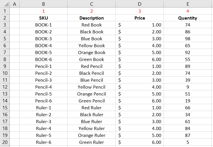
Notice that Table does not start from Cell A1. This is to illustrate when choosing the table in the Vlookup it does not require to start at the left of the sheet, but rather of the left of the table of array.
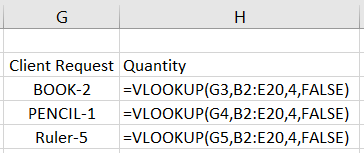
The Client wants the following three items Quantity. Book-2, Pencil-1, and Ruler-5. Your formula when entering it Manually will look like this:
When looking at the full view you will see excel tries and shows you exactly what data you enter by color coding each section of the formula cell with the same color:
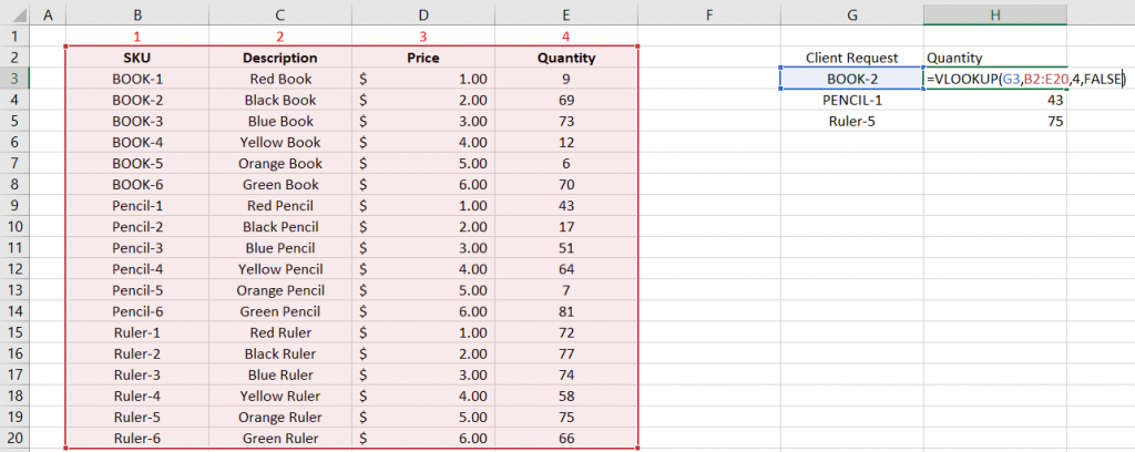
Notice that the Column count 4 is the fourth column on your Table selected.
The problem with the Vlookup formulas is I manually typed each one in thus it took me more time than what it should have. Especially if there are many more than three SKU’s to search for. The thing with Excel is it tries and helps you do your work faster and more efficiently. What happens is you can enter the Formula once and Drag it down to auto adjust the columns below trying to predict which information you are going to fill in.
Table_Array Common Mistake
The problem is it will auto adjust all your values. Let’s see an example with a few more SKU’s where Excel assisted with auto-completing your Formulas.
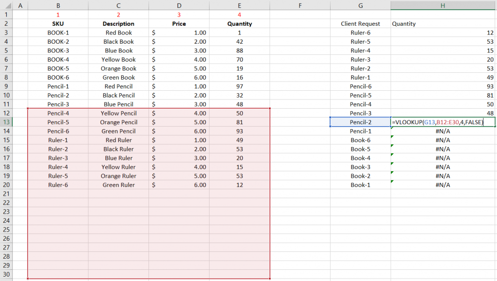
As you can see excel adjusted the location of the Vlookup array as well as the Vlookup Value. Thus it got to a point where the Lookup Value was not part of the Array any more and could not find data to return.
To get around this there is two solutions that works very well depending on the situation. The First is the simplest and it is selecting the complete Columns instead of only a Selection.
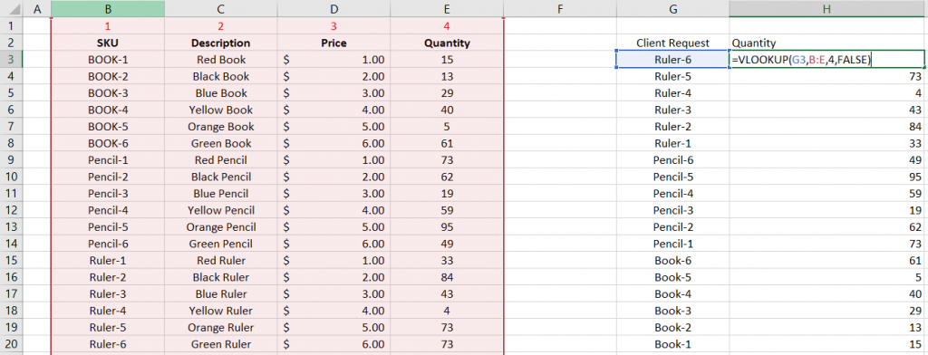
As you can see this will go through every cell in the B column that has a value. The problem I personally have with this way is every cell that had a value previously will also be worked through as there is a difference between a Empty cell (A cell that had Data Previously) and a NULL Value Cell (A Cell that never had Data).
The way to fix this is to Select all ROWS that is Empty and actually right clicking and Deleting those rows. As a test try this with your existing Excel Sheets and look at the size difference of the file before and after.
Absolute Values
The Second way of getting around the auto adjust of Excel is by telling excel not to change certain values. This gets done by adding a $ (Dollar Sign) in front of the values is should not change before dragging the formula down.
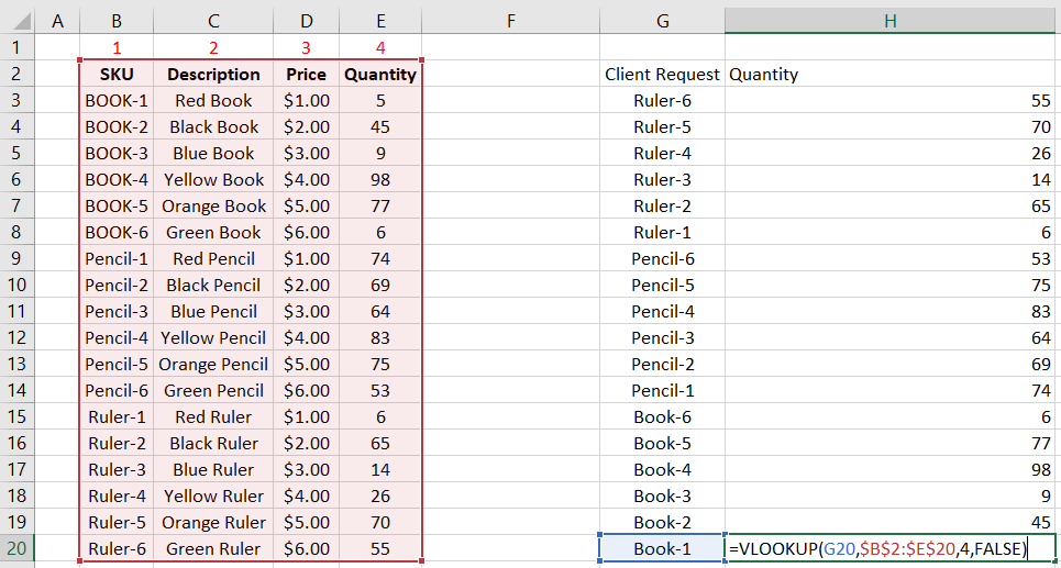
As per above the Formula shows the table_array and a $ (Dollar sign) in front of every value that can change. This now told Excel don’t change the Values when auto adjusting.
The absolute values comes in very handy with other types of functions as well.
Duplicate Values
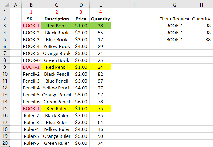
Lastly, Vlookup only looks up one Value at a Time and ends when it finds that Value. If you have multiple Lookup Values that are the same it will only return the first one that it matches with anything after that will be ignored.
