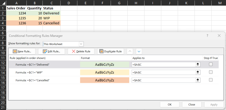
Efficient data visualization is crucial for making sense of complex datasets in Excel. One powerful technique that aids in this process is conditional formatting, which allows users to dynamically highlight rows based on specific cell values. This not only makes patterns and trends stand out but also provides an instant visual representation of data relationships. In this blog post, we’ll guide you through the process of using conditional formatting to highlight entire rows in Excel, based on the value of a specific cell.
Understanding Conditional Formatting
Conditional formatting in Excel enables you to apply different formatting styles to cells based on certain conditions or rules. It’s a valuable tool for quickly identifying important data points, outliers, or trends in your dataset. When applied to entire rows, conditional formatting can transform your spreadsheet from a sea of numbers into an insightful visual aid.
Step-by-Step Guide
Here’s a step-by-step guide to using conditional formatting to highlight rows in Excel based on the value of a specific cell:
Step 1: Select the Data Range
Start by selecting the range of data where you want to apply the conditional formatting. This range should include the column with the specific cell value you want to base the formatting on, as well as the other columns you want to highlight.
Step 2: Access Conditional Formatting
Navigate to the “Home” tab on the Excel ribbon. In the “Styles” group, locate and click on the “Conditional Formatting” button. A dropdown menu will appear.
Step 3: Create a New Rule
From the dropdown menu, select “New Rule.” This will open the “New Formatting Rule” dialog box.
Step 4: Specify the Rule Formula
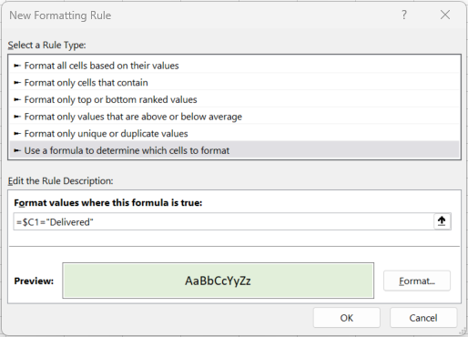
Choose the option that says “Use a formula to determine which cells to format.” In the input field below, enter the formula that checks the value of the specific cell. For example, if your specific cell is in column E and you want to highlight rows where the value in column E is “X,” the formula should be: =$E1="X". The dollar sign before “E” makes sure the column reference doesn’t change as you apply the rule to different rows.
Step 5: Define Formatting Style
Click on the “Format” button to open the “Format Cells” dialog box. Here, you can customize the formatting style for the highlighted rows. You can change the font color, fill color, borders, and more. Experiment with different styles to find what works best for your data visualization needs.

Step 6: Apply the Rule
After defining the formatting style, click “OK” to close the “Format Cells” dialog box. You’ll now be back in the “New Formatting Rule” dialog box. You can preview how your selected formatting style will look by using the preview area in the dialog box.
Step 7: Confirm and Enjoy
Click “OK” in the “New Formatting Rule” dialog box to apply the conditional formatting rule. Voilà! The rows that meet your specified condition will now be dynamically highlighted based on the formatting style you chose.

Formatting in Excel is a game-changer when it comes to enhancing data visualization. By highlighting entire rows based on the value of a specific cell, you can quickly uncover insights, trends, and relationships within your data. This technique not only improves data interpretation but also enables you to make informed decisions more effectively. So, go ahead and give conditional formatting a try in your Excel spreadsheets – your data will thank you for the visual makeover!
