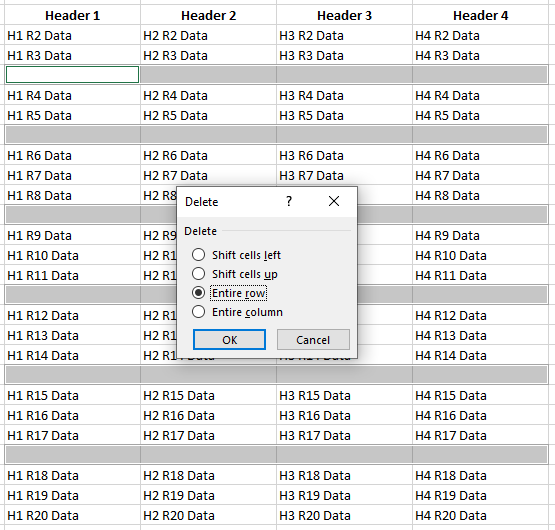
Removing Blank lines in Excel can be done in a few different ways.

1. Create a Filter
2. Create a Table
3. Special Select

Create a Filter

Start by selecting the complete range of data that you want to remove data on. On the “Home” Menu find “Editing“, “Sort & Filter”, and choose “Filter“.

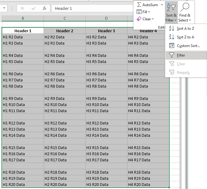
Now click any one of the Dropdown buttons on the header, and choose “Sort A to Z” or “Sort Z to A“.

Create a Table

Select any Cell with data on the Sheet. Press “CTRL + T” . This will open a new “Dialog box” where you can Highlight the complete Data Set. Also, Tick the option “My Table has Headers“

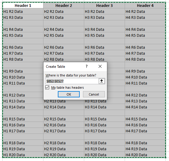
Now follow the same step as Filtering, click any one of the Dropdown buttons on the header, and choose “Sort A to Z” or “Sort Z to A“

Filter VS Table

The big difference between the Filter and Table option can be seen after sorting a Table. At the bottom of the table, you will see the rows still showing which means the Rows are not really empty:

Special Select

Lastly, select the complete range then Press F5. On the Go To Dialog box choose Special…

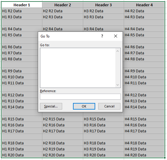
Choose Blanks on the Go To Special and Press OK

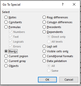
This will Highlight all Cells with No Data in them. Press CTRL + Minus (-) and select Entire Row then press OK. This will keep the Data in the same Order but remove all the Blanks.